Applied Bayesian Data Analysis
Building blocks
Building blocks
Concepts
- Posterior, predictive prior and posterior
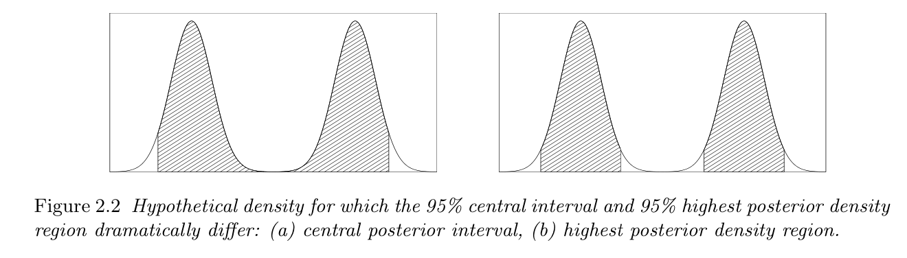
- Compatibility intervals
- Bernoulli, Binomial, Poisson, Exponential, Normal
Representing distributions
A generative model uses:
- Prior distribution of parameters $\theta$
- conditional distribution of observations $y | \theta$
Example — Beta-Bernoulli:
\begin{align} \theta &\sim Beta(1, 1) \\ y|\theta &\sim Bernoulli(\theta) \end{align}Representing distributions
A generative model defines:
- Prior predictive distribution of $y$: $$p(y)= \int p(y, \theta) d\theta$$
- Posterior distribution of $\theta$: $$p(\theta|y) = \frac {p(\theta)p(y|\theta)} {\int p(\theta)p(y|\theta)d\theta} \propto p(\theta)p(y|\theta)$$
- Posterior predictive distribution of $\tilde y$: $$p(\tilde y | y) = \int p(\tilde y|y, \theta)p(\theta|y)d\theta = \int p(\tilde y|\theta)p(\theta|y)d\theta$$
Approximation by samples
- In some models, distributions are available in closed form. Example — Beta-Bernoulli:
- In most models, no closed form. We approximate distributions by samples.
- How can we summarize the posterior in a few numbers. And why should we?
Summarizing samples
- Summary statistics
- Point estimates
- Compatibility intervals
Summary statistics
- Mean, standard deviation(, skew, kurtosis, ...)
- Fully defines known distributions
- Gives information about shape
- Can be misleading: Beta, Normal, Gamma
Point estimates
- Mean: $\mathrm{mean} = \mathbb{E}(x) = \int x p(x) dx$
- Median: $\Pr(x \le \mathrm{median}) = \Pr(x \ge \mathrm{median})$
- Mode: $\mathrm{mode} = \arg \max p(x)$

Compatibility intervals
- Central intervals — ‘quantiles’
- Highest posterior density regions
Some ‘standard’ models
Continuous
- Normal - the ‘standard’ distribution
- Exponential — time between phone calls
- Gamma — time between scheduled buses
- ...
Normal distribution
Sum of many random variables: Galton board
Example: human height and weight
Height and weight Kaggle dataset


Poisson model
- Conditional probability: $$p(y|\theta)=\frac {\theta^y e^{-\theta}} {y!},\mbox{ for }y=0,1,2,...$$
- Rate and exposure
$$y_i \sim \mathrm{Poisson}(x_i\theta)$$
- $x_i$ — exposure, known
- $\theta$ — rate, unknown
Example: cancer rates
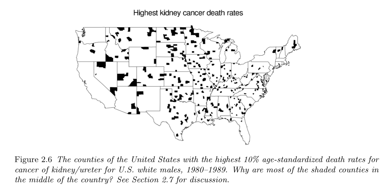
Example: cancer rates
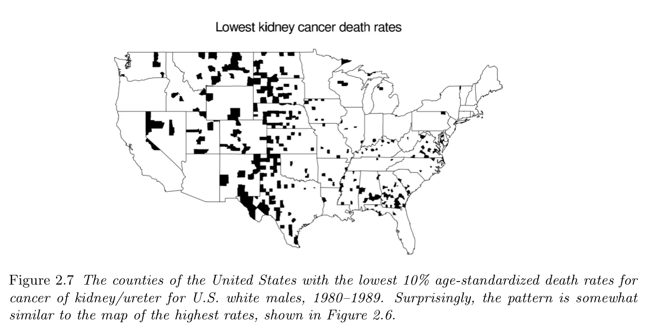
Example: cancer rates
Model
- Sampling distribution: $y_i \sim \mathrm{Poisson}(10n_j\theta_j)$
- Prior distribution: $\theta_j \sim \mathrm{Gamma}(20, 430\,000)$
- Posterior disribution: $\theta_j|y_j \sim \mathrm{Gamma}(20+y_j, 430\,000 + 10n_j)$
- Small county: mostly prior
- Large county: mostly observations
Readings
- Statistical rethinking — chapters 3 and 4.
- Bayesian Data Analysis — chapter 2.
Hands-on
- Summarizing the posterior, on girl birthrate study.
- Model zoo, in Pluto notebook.