Applied Bayesian Data Analysis
Approximate computations
Concepts
- Quadrature
- Monte Carlo methods, Markov chain Monte Carlo
- Automatic differentiation
Approximate computations
Concepts
- Quadrature
- Monte Carlo methods, Markov chain Monte Carlo
- Automatic differentiation
Approximate Bayesian computation
- We need:
- posterior distribution $p(\theta|y)$
- posterior predictive distribution $p(\tilde y|y)$
- We use posterior to compute integrals:
- mean
- variance
- condifence intervals
- expected utility
- We approximate the posterior with samples
Numerical integration — Quadrature
- Monte Carlo approximation: $$E(h(\theta)|y) = \int h(\theta)p(\theta|y)d(y)d\theta \approx \frac 1 S \sum_{s=1}^S h(\theta^s)$$
- Low of large numbers for independent samples: $$\lim_{S\to \infty} \frac 1 S \sum_{s=1}^S h(\theta^S) = E(h(\theta)|y)$$
Monte Carlo methods
- Inverse transform sampling
- Rejection sampling
- Importance sampling
Inverse transform sampling
- Given CDF $F(x)$ (and inverse CDF $F^{-1}(x)$)
- Sample $U$ from $[0, 1]$ uniformly
- Compute $v = F^{-1}(U)$.
Helps sample from library distributions.
Rejection sampling
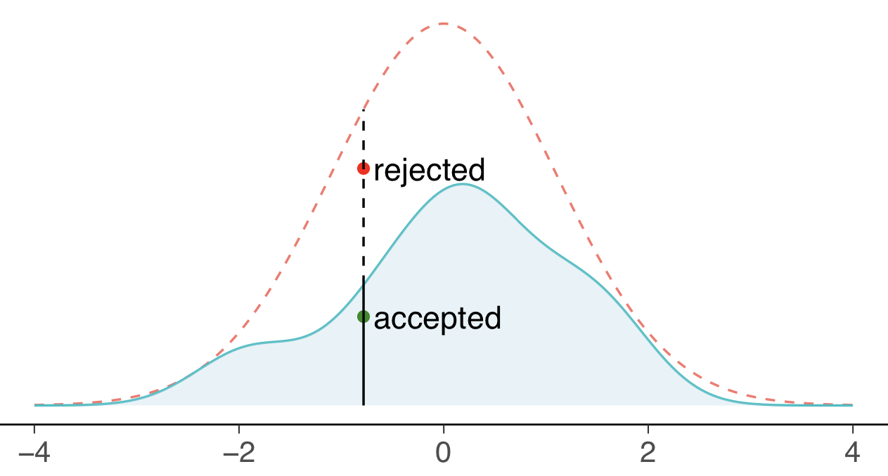
- Target $q(\theta|y)$, proposal $g(\theta)$
- Draw $v$ from $g(\theta)$
- Draw $u$ uniformly from $[0, 1]$
- Accept if $\frac {q(\theta|y)} {Mg(\theta)} > u$
Useful for 1-dimensional distributions.
Importance Sampling
- Target $q(\theta|y)$, proposal $g(\theta)$
- Draw $v$ from $g(\theta)$
- $E(h(\theta|y)) = \frac {\sum_{i=1}^S w_s h(\theta^s)} {\sum_{i=1}^S w_s}$ where $w_s = \frac {q(\theta^s)} {g(\theta^s)}$
- For some $\theta$, $q(\theta)$ can be higher than $g(\theta)$
With a good proposal IS is more efficient than RS.
Markov Chain Monte Carlo
- Draws samples from Markov chain
- Easy to sample
- Chain equilibrium samples from posterior
- (👎) samples are dependent
- (👎) efficient chains can be hard
Markov chain
- $\theta^1,\theta^2,\ldots$; $\theta^t$ depends only on $\theta^{(t-1)}$
- Chain starts with starting point $\theta^0$
- Transition distribution $T_t(\theta^t|\theta^{t-1})$ (may depend on $t$)
- By choosing a suitable transition distribution, the stationary distribution of Markov chain is $p(\theta|y)$
Markov chain
- Transition: $\theta^{t+1}|\theta^{t} \sim \mathcal{N}(0.5x^{t}, 1.0)$
- Posterior: $\theta \sim \mathcal{N}(0, 1.33)$
Metropolis Hastings
- Initialize:
- Pick $x_0$
- Set $t = 0$
- Iterate:
- Generate candidate $x'$ according to $g(x' \mid x_t)$.
- Calculate the acceptance probability $A(x', x_t) = \min\left(1, \frac{P(x')}{P(x_t)} \frac{g(x_t \mid x')}{g(x' \mid x_t)}\right)$
- Accept or reject:
- generate a uniform random number $u \in [0, 1]$
- if $u \le A(x' , x_t)$, then accept: $x_{t+1} = x'$;
- if $u > A(x' , x_t)$, then reject: $x_{t+1} = x_{t}$.
- Increment: $t = t + 1$.
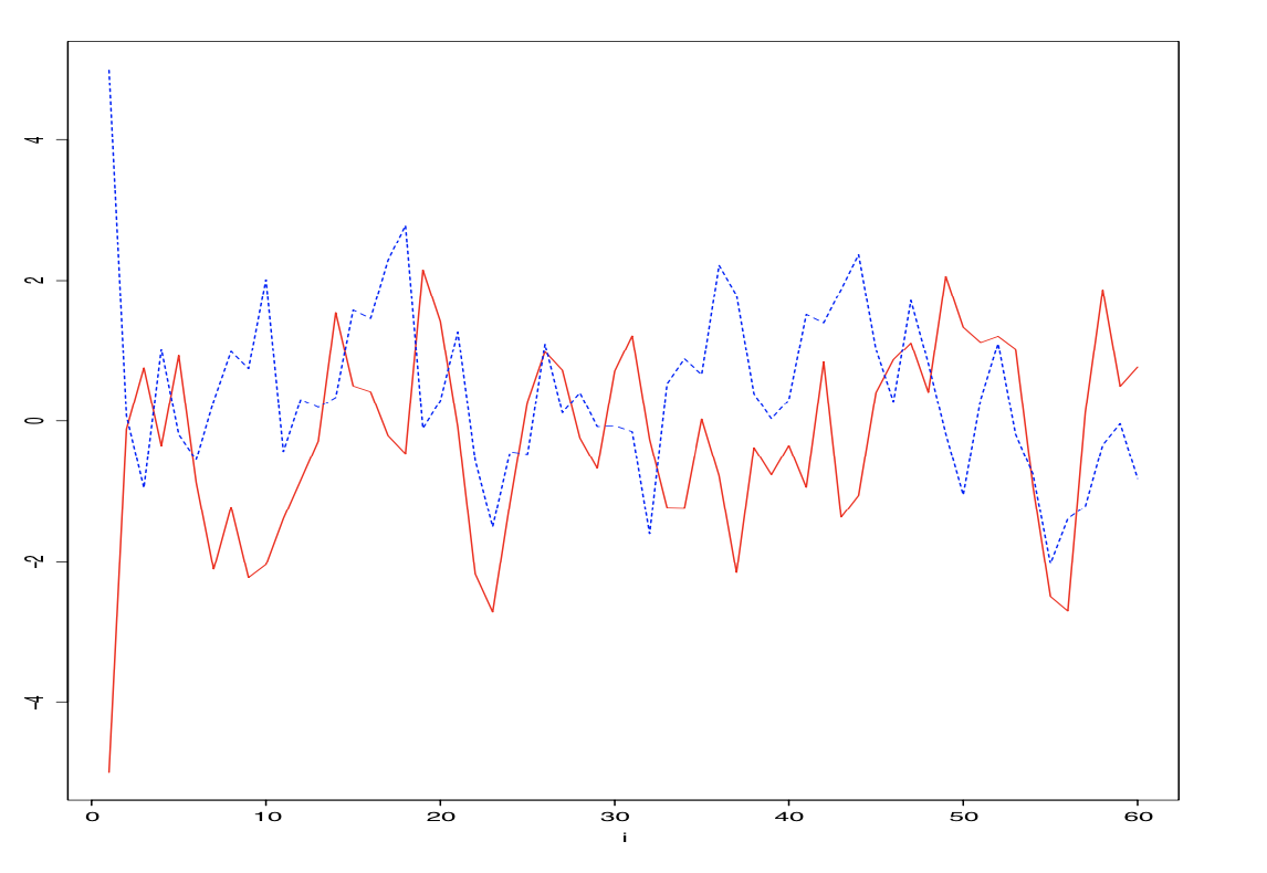
Metropolis-Hastings: mixing of chains

Automatic differentiation
- We can make sampling faster by using gradients.
- We need the gradient of the model $p(x, y)$ by it's parameters $x$: $$\nabla_x p(x, y)$$
- How do we get it?
Differentiation

- Slope of the function's tangent
- $f'(x) = \lim\limits_{h \to 0} \frac {f(x+h) - f(x)} {h}$
- also $\frac {df} {dx}$ (Leibniz's notation)
- Partial derivatives: $\frac {\partial f(x_1, x_2, ..., x_n)} {\partial x_i}$
Differentiation rules
- Constant rule: if $f(x)=C$ then $f'(x)=0$
- Sum rule: $(f(x) + g(x))' = f'(x) + g'(x)$
- Product rule: $(f(x)g(x))' = f'(x)g(x) + f(x)g'(x)$
- Quotient rule: $\left(\frac 1 {f(x)}\right)'=-\frac {f(x)'} {f(x)^2}$
- Chain rule: $f(g(x))' = f'(g(x))g'(x)$
Differentiation examples
$$1' = 0$$ $$x' = 1$$ $$\left(x^2\right)'= xx' + x'x = 2x$$ $$sin(x)' = cos(x)$$ $$tan(x)' = \left( \frac {sin(x)} {cos(x)}\right)' = \frac {sin^2(x) + cos^2(x)} {cos^2(x)} = \frac 1 {cos^2(x)}$$ $$...$$How do computers differentiate?
- Numerical differentiation
- Symbolic differentiation
- Algorithmic differentiation
Numerical differentiation
- Choose $h$
- Compute $f(x)$
- Compute $f(x+h)$
- Return $\frac {f(x+h) - f(x)} h$
Problems
- $h$ too large — truncation error (שגיאת קיטום)
- $h$ too small — roundoff error (שגיאת עיגול)
Symbolic differentiation
- Represent function symbolically.
- Apply differential rules.
Problems
- Loops, conditionals, recursion.
- Code swell:
\begin{equation} \begin{aligned} \left( \frac {\log(x) + \exp(x)} {\log(x)\exp(x)}\right)' = & -\frac {\exp(-x)(\log(x)+\exp(x))} {\log(x)} \\ & -\frac {\exp(-x)(\log(x)+\exp(x))} {x\log^2(x)} \\ & + \frac {\exp(-x)\left(\exp(x) + \frac 1 x\right)} {\log(x)} \end{aligned} \end{equation}
Algorithmic differentiation
- NOT symbolic differentiation
- NOT numerical differentiation
- differentiates ANY code
- computation costs of $f'(x)$ and $f(x)$ are similar
Algorithmic differentiation
						function f(a, b)
						  c = a*b
						  d = sin(c)
						  d
						end
						function f(a, da, b, db)
						  c, dc = a*b, da*b + a*db
						  d, dd = sin(c), dc * cos(c)
						  d, dd
						end
Program trace
f.jl
						function f(a,b)
						  c = a*b
						  if c > 0
						    d = log(c)
						  else
						    d = sin(c)
						  end
						  d
						end
f(2, 3)
						a=2, b=3
						c=a*b=6

						d=log(c)=1.791


						d=1.791
f(2, 3), df(2, 3)/da
						a=2, b=3, da=1, db=0
						c=a*b=6,  dc=da*b + a*db=3

						d=log(c)=1.791, dd=dc*(1/c)=0.5


						d=1.791, dd=0.5
Hamiltonian Monte Carlo
Hamiltonian MC is based on statistical physics:
- Velocity `$v$` is added to the parameters describing the system.
- Energy of the system consists of potential and kinetic parts: $$ E(\pmb{x}, \pmb{v}) = U(\pmb{x}) + K(\pmb{v}), \qquad K(\pmb{v}) = \sum_i \dfrac{m \, v^2_i}{2} $$
- Velocities `$ \pmb{v} $` and positions `$ \pmb{x} $` have independent canonical distributions: $$ p(\pmb{x}, \pmb{v}) \propto \exp\left( \frac{-E(\pmb{x}, \pmb{v})}{T} \right) = \exp\left( \frac{-U(\pmb{x})}{T} \right) \, \exp \left( \frac{-K(\pmb{v})}{T} \right) \propto p(\pmb{x}) \; p(\pmb{v}). $$
- So once we can sample from joint distribution `$p(\pmb{x}, \pmb{v})$`, we also can sample `$\pmb{x}$` by ignoring computed velocities `$\pmb{v}$`.
- Automatic differentiation is needed to compute $\nabla_U$ to simulate particle motion.
Readings
- Pattern Recognition and Machine Learning — Chapter 11: Sampling Methods.
- Bayesian Data Analysis — Part III: Advanced Computation.
- Statistical rethinking — Chapter 9: Markov Chain Monte Carlo.