Applied Bayesian Data Analysis
Hierarchical models
Hierarchical models
Concepts
- Hyperprior
- Pooled vs. separate
- Group exchangeability
Inspiration
Box of marbles, from flat to hierarchical
Applied Bayesian Data Analysis
Hierarchical models
Concepts:
- Separate model, pooled model, hyperparameters
- Hierarchical normal model
- Exchangeability
Hierarchical model basics
- Many models represent 'groups'
- Parameters are shared inside groups
- Parameters of different groups are related
- Represented by hierarchical models
- Parameters of parameters are called hyperparameters
CVD treatment example
- n hospitals
- CVD treatment in each hospital
- patients $y_{ij}$ at $j$th hospital survive with prob. $\theta_j$
- $\theta_j$ are related, via hyperparameter $\tau$
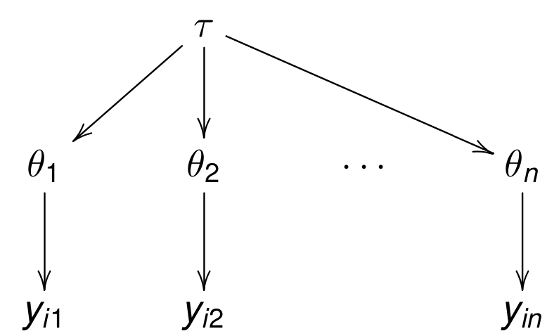
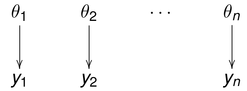
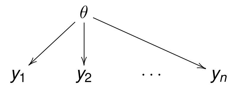
Separate, pooled, hierarchical
Separate (overfit)
Pooled (bias)
Hierarchical
Probabilities
- hyperprior $p(\tau)$
- priors on parameters $p(\theta_j|\tau)$
- observations $p(y_{ij}|\theta_j)$
Joint posterior: $$p(\theta, \tau|y) \propto p(y|\theta)p(\theta|\tau)p(\tau)$$
Example: risk of tumor in group of rats
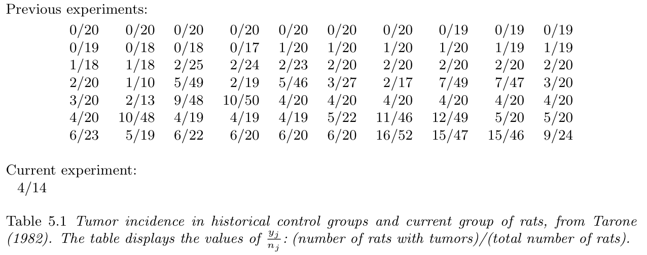
Tumor in rats: population prior
- Prior: $Beta(\alpha, \beta)$, posterior: $Beta(\alpha + 4, \beta + 10)$
- Estimate prior from $\frac {y_j} {n_j}$: $\alpha=1.4$, $\beta=8.6$
- Posterior: $Beta(5.4, 18.6)$
Problems?
Population prior: problems
- Same prior for first 70 experiments: double counting?
- Point estimate is not Bayes!
- Prior must be known before data. What is known before data?
Example: eight schools
- students had made pre-tests PSAT-M and PSAT-V
- part of students were coached
- linear regression was used to estimate the coaching effect $y_j$ for the school $j$ (could be denoted with $\bar{y}_{.j}$, too) and variances $\sigma_j^2$
- $y_j$ approximately normally distributed, with variances assumed to be known based on about 30 students per school
- data is group means and variances (not personal results)
Eight schools: data
| School | effect, $y_j$ | error, $\sigma_j$ |
|---|---|---|
| A | 28 | 15 |
| B | 8 | 10 |
| C | -3 | 16 |
| D | 7 | 11 |
| E | -1 | 9 |
| F | 1 | 11 |
| G | 18 | 10 |
| H | 12 | 18 |
Eight schools: model
\begin{aligned} \mu & \sim \mathrm{Normal}(0, 10) \\ \tau & \sim \mathrm{LogNormal}(0, 10) \\ \eta_i & \sim \mathrm{Normal}(0, 1) \\ \theta_i & = \mu + \tau\eta_i \\ \mathit{effect}_i & \sim \mathrm{Normal}(\theta_i, \mathit{error}_i) \end{aligned}Results in notebook.
Exchangeability
- Justifies why we can use
- a joint model for data
- a joint prior for a set of parameters
- Less strict than independence
Exchangeability: definition
- Parameters $\theta_1,\ldots,\theta_J$ (or observations $y_1,\ldots,y_J$) are exchangeable if the joint distribution $p$ is invariant to the permutation of indices $(1,\ldots,J)$
- e.g. $p(\theta_1,\theta_2,\theta_3) = p(\theta_2,\theta_3,\theta_1)$
- Exchangeability implies symmetry: If there is no information which can be used a priori to separate $\theta_j$ form each other, we can assume exchangeability. ("Ignorance implies exchangeability")
Results of experiments can be different
-
We know that:
- the experiments have been in two different laboratories
- the other laboratory has better conditions for the rats
- a priori experiments are exchangeable
Hierarchical exchangeability
Example: hierarchical rats example
- all rats not exchangeable
- in a single laboratory rats exchangeable
- laboratories exchangeable
- $\rightarrow$ hierarchical model
Partial or conditional exchangeability
- Conditional exchangeability:
if $y_i$ is connected to an additional information $x_i$, so that $y_i$ are not exchangeable, but $(y_i,x_i)$ exchangeable use joint model or conditional model $(y_i|x_i)$. - Partial exchangeability:
if the observations can be grouped (a priori), then use hierarchical model
Exchangeability and independence
- The simplest form — conditional independence: $$p(x_1,\ldots,x_J|\theta)=\prod_{j=1}^J p(x_j|\theta)$$
- Let $(x_n)_{n=1}^{\infty}$ to be an infinite sequence of exchangeable random variables. De Finetti's theorem: there is some random variable $\theta$ so that $x_j$ are conditionally independent given $\theta$.
- Joint density $x_1,\ldots,x_J$ is a mixture: $$p(x_1,\ldots,x_J)=\int \left[\prod_{j=1}^J p(x_j|\theta)\right]p(\theta)d\theta$$
Dependent but Exchangeable
- A six sided die with probabilities (a finite sequence!)
$\theta_1,\ldots,\theta_6$
- without additional knowledge $\theta_1,\ldots,\theta_6$ exchangeable
- due to the constraint $\sum_{j=1}^6\theta_j$, parameters are not independent and thus joint distribution can not be presented as iid mixture
Readings
- Bayesian Data Analysis — chapter 5.
- Statistical rethinking — chapter 13.
- Probabilistic Models of Cognition — chapter 12.
Hands-on
- 8 schools
- Reed frogs